A Stochastic Game Framework for Groundwater Markets

Regulatory frameworks such as California’s Sustainable Groundwater Management Act (SGMA) have accelerated the need for market-based mechanisms to manage aquifer depletion. In (Cialenco & Ludkovski, 2025) we introduce a stochastic dynamic game model to analyze these emerging groundwater markets, where stakeholders (farmers) optimize production and trading decisions under physical and regulatory constraints.

The Model

We model the interaction as a non-cooperative game among \(J\) economic agents who each grows several crops. Each agent $j$ maximizes the expected utility of their profit and loss (P&L), denoted as \(L_j(t)\). The P&L is derived from agricultural production revenue and proceeds from water trading \(\psi_j(t)\) at the market price \(p(t)\):

\[L_{j}(t):=\sum_{k=1}^{K}\overline{f}_{j}^{k}(t,\varphi_{j}^{k})\cdot\varphi_{j}^{k}(t)+\psi_{j}(t)\cdot p(t)\]

Here, \(\varphi_{j}^{k}\) represents the quantity of crop $k$ produced, and \(\overline{f}_{j}^{k}\) is the net profit per unit. The system dynamics are driven by exogenous groundwater recharge $R(t)$ and the ability of agents to “bank” water for future periods. The water available to agent $j$ evolves according to:

\[W_{j}(t+1)=W_{j}(t)+\theta_{j}R(t+1)-C_{j}(t)-\psi_{j}(t)\]

where \(\theta_j\) is the agent’s share of recharge and \(C_j(t)\) is water consumption. The key state process \((R_t)\) is assumed to follow a discrete-state Markov chain.

Equilibrium Dynamics

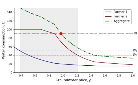
In a single-period static setting, the market clears at a Pareto optimal price $p^\circ$, defined by the intersection of aggregate demand and total available water.

Figure 1: Left: Groundwater consumption $C_j(p)$ as a function of price. Right: Optimal production quantities $\varphi_{j}^{k,\ast}(p)$.

A fundamental result is any price $p$ yields a Nash Equilibrium.

Multiple Periods

However, in a multi-period setting, the option to bank water introduces non-zero-sum game effects. gents must balance current profits against future scarcity, with their banking decisions $b_j(t)$ impacting future market prices for all participants. The Nash Equilibrium is characterized by the fixed point of the agents’ best response curves, $b_j^* = B_j(b_{-j}^*)$.

Figure 2: Best response curves $\bar{b}_{-j} \mapsto B_j(\bar{b}_{-j})$ for a two-period market. The intersection marks the equilibrium banking strategies.

This framework highlights that while banking generally benefits individual agents by smoothing intertemporal shocks, rational smoothing behavior can negatively impact competitors by altering future water valuations.

In a forthcoming post we examine more closely dynamic effects from banking over multiple periods.