Dynamic Phenomena in Multi-period Groundwater Markets

Following up on our earlier post we discuss multi-period groundwater markets.

The Model

We model the groundwater market as a non-cooperative game among $J$ economic agents who each generate profits by irrigating their fields with groundwater according to a profit function $G_j(C)$. Each period, conventionally corresponding to a calendar year, agent $j$ gets an allocation $R_j(t)$ (measured in acre-feet), which they can either pump or trade with other agents. The allocations $R_j$ are stochastic and driven by the recharge process ${R(t)}$, which is viewed as exogenous and can be linked to surface precipitation. Below we concentrate on proportional allocations, $R_j(t) = \theta_j R(t)$ for a constant $\theta_j$.

The key ingredient in the dynamic model is the opportunity for individual stakeholders to bank their pumping rights across seasons. Banking reduces available water today and increases groundwater available next period, decoupling newly allocated rights from water $W_j(t)$ available for pumping:

\[W_j(t+1) = b_j(t) + R_j(t+1) \quad t=0,\ldots, T-1.\]

The assumption that $b_j(t)$ is non-negative is essential and implies that agents cannot borrow from their future allocations, but must first build up pumping reserves. In turn, in the present period, available water is composed of consumption $C_j(t)$, trading $\psi_j(t)$ and banking:

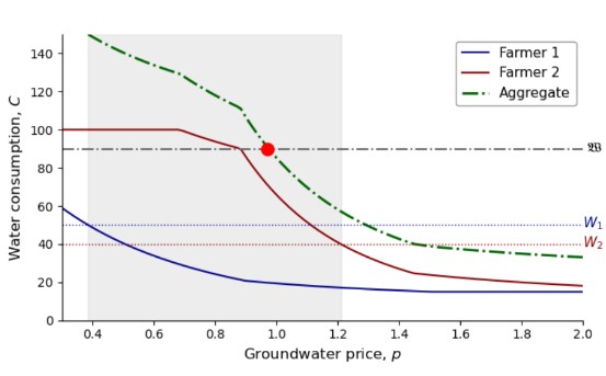
\[W_j(t) = C_j(t) - \psi_j(t) + b_j(t)\]

with the market clearing condition $\sum_{j=1}^J \psi_j(t) = 0$. Each agent $j=1,\ldots,J$ selects a strategy (aka control) $\pi_j(t) = \big(C_j(t), \psi_j(t)\big)$ at each period $t$ from the action set \(\mathcal{A}_j(\mathbf{W}):= \mathcal{C}_j(t) \times [-\sum_{i\neq j} W_j(t), {W}_j(t)]\)

---

The state process is ${\mathbf{W}(t), R(t)}$ which tracks the groundwater rights vector as well as the recharge regime that is assumed to follow a Markov chain. Each agent $j$ maximizes her expected risk-adjusted payoff

\[A_j(\pi_j, \pi_{-j},p; 0, \mathbf{w}, r) = \mathbb{E}^{\pi} \Big[\sum_{s=0}^T U_j(L_j(s; \pi_j(s),p(s))) \mid \mathbf{W}(0) = \mathbf{w}, R(0) = r\Big], \qquad L_j(t) := G_j(t,C_j(t)) + \psi_j(t) \cdot p(t),\]

where $U_j$ is a concave utility function.

---

We consider only Markovian policies, so that the joint process $(\boldsymbol{W}(t), \mathbf{R}(t))$ is Markov, i.e., has no memory. In equilibrium, the value of the continuation game of the agent $j$, $A_j(\pi_j, \mathbf{\pi}_{-j}, p)$ is maximized in $\pi_j$ for each $j$. Denote the best-response continuation value as

\[\mathcal{V}_j( \pi_{-j}, p; t, \mathbf{w}, r) := \sup_{\pi\in\mathscr{S}_j} A_j(\pi, \mathbf{\pi}_{-j}, p; t, \mathbf{w}, r).\]

Then the game value for a Sub-Game Perfect Markov Nash Equilibrium can be recursively constructed by

\(\mathcal{V}_j(\mathbf{\pi}_{-j}, p; t, \mathbf{w}, r) = \max_{C_j, \psi_j}\Big[U_j \bigl( G_j(t, C_j) + \psi_j p \bigr)+ \mathbb{E}^{\mathbf{\pi}}[ \mathcal{V}_j(\mathbf{\pi}_{-j}^\circ, p^\circ; t+1, \mathbf{w} + \mathbf{R}(t+1) - \mathbf{C} - \boldsymbol{\psi}, R(t+1) ) \mid \mathbf{W}(t) = \mathbf{w}, R(t) = r] \Big]\) The equilibrium groundwater price $p^\circ$, trading $\psi^\circ_j$ and consumption volumes $C^\circ_j$ are obtained according to the 1-period model detailed in (Cialenco & Ludkovski, 2025).

In the case study below we consider recharge distribution $R(t) \in { 40, 75, 95}$ interpreted as droughts, average precipitation and wet years. We consider a finite planning horizon of $T=25$ periods, with 2 farmers whose profits $G_j(C)$ as a function of water consumed $C$ are depicted in Figure 1. In line with standard economic frameworks, profits are concave, in particular they are more concave for Farmer 2 than for Farmer 1.

Emerging phenomena

The primary impact of banking is smoothing of consumption, visualized in Figure 2. The highly volatile recharge time-series (the dotted curves $R_j(t)$) transform into the much smoother trajectories of consumption $C^\circ_j(t)$. This is achieved through stakeholders banking some of their rights, and then drawing them down during droughts, see the drop in $b^\circ_j(19)-b^\circ_j(18)$.

Observe how both farmers quickly bank up a significant reserve (middle panel), which allows them to withstand a single year of drought (year $t=4$) with minimal impact on consumption (bottom panel) and hence profits. Drought does substantially deplete banked allocations, so after multiple dry years, consumption would eventually be affected, see the three consecutive years of drought at $t=19, 20, 21$, with almost no reserves left after the second year and consumption $C^\circ_j(21)$ plummeting accordingly.

The equilibrium groundwater price $p^\circ(t)$ (top panel) is computed endogenously and reflects the current scarcity: $p^\circ(t)$ is high during droughts and low during wet years. Towards the end of the problem horizon, $p^\circ(t)$ drops as farmers race to spend down their reserves before the horizon $T$.

As another endogenous feature we observe that while Farmer 1 buys rights from Farmer 2 during regular or wet years, Farmer 1 sells rights $\psi_1(t)>0$ during droughts, so the trading dynamically and path-dependently adjusts to market conditions.

Figure 3 shows how banking shifts the distribution of one-step profits relative to the base situation where banking is not allowed. In the latter case, farmers can only pump and trade whatever is allocated in the present year. In our simulation, we assume that recharge is a Markov chain with 3 states, hence the no-banking settings leads to discrete profit distribution with 3-point support. The respective probabilities, indicated by the red bars correspond to the stationary distribution $\vec{\pi}$ of ${ R(t)}$.

With banking, their profits have a non-trivial distribution, concentrated in $v_1 \in [60,74]$ and $v_2 \in[52,59]$, which is generally more than during the medium-precipitation year and less than during the wet year. Opportunity to bank dramatically cuts down profit variability. Compared to the case of no banking, the standard deviation is reduced by 58% for Farmer 1 and by 62% for Farmer 2. In particular, by building up reserves, farmers avoid the losses associated with droughts. There is $\pi_1 = 1/9 = 11.1\%$ of drought and without banking, the respective minimal recharge leads to revenues of less than 40. With banking, the 95% profit quantile is 60.23 for Farmer 1 and 50.13 for Farmer 2 and there is about 0.5% chance of earning less than 40. Figure 2 also shows how the precautionary motive to bank is driven by risk-aversion: in the base case the risk averse agents with log-utility construct a tighter and less-skewed profit distribution compared to risk-neutral farmers.

Our model also allows to study the role of groundwater rights allocation mechanism on the market. For example, suppose that instead of Farmer 1 getting 60% of the rights and Farmer 2 getting 40% (corresponding to allocation vector $[(24,16), (45,30), (57,38)]$), the allocation is flipped to the 40%/60% ratio with allocation vector $[(16,24), (30,45), (38,57)]$. Figure 4 shows that this leads to a substitution effect in banking: Farmer 2 who now has more rights will bank more, and Farmer 1 banks less. In effect, the “richer” Farmer also takes on the role of being the leading “banker”. Note that implicitly there is also a wealth transfer: profits of Farmer 2 go up and those of Farmer 1 down, in particular because the latter now has to buy more rights from the former. Figure 3 also shows a junior/senior allocation $[(30,10), (45,30), (45, 50)]$, where this shift in banking roles is even more exacerbated. In that third scenario, Farmer 2 bears the brunt of the exogenous recharge fluctuations and as the result is more incentivized to smooth them out.

In the boxplots of Figure 4, each dot represents a scenario (1000 scenarios total) and the colors represent the current regime $R(t)$. As expected, during droughts (red dots), banking is reduced, while it is highest during wet years (grey dots).